Quantum random walk is the analog to the classical random walk. In quantum random walk, many interesting phenomena distinguished from its classical counterpart can be found and studied. Thus, a comprehensive software package for the simulation of quantum random walk is needed.

We developed the Second Quantization Quantum Walk (Github) package in Mathematica that supports symbolic specification of the quantum walker in the form of second quantization ladder operators.

It supports symbolic Wick expansion of operators and automatic Hamiltonian construction. GPU acceleration is supported on machines with CUDA installed. Various of types of auxiliary functions are defined for postprocessing of simulation data.

(The code snippet here is a complete program for simulating a 2D quantum walk.)

$$ \def\ket{\left| 0 \right\rangle} \def\ketl{\left| l \right\rangle} \def\ketlp{\left| l+1 \right\rangle} \def\ketlm{\left| l-1 \right\rangle} \def\ladup{a^{\dagger}} \def\laddown{a} \def\pnum{n^} $$

Second quantization formulation of quantum walk

For simplicity, consider a quantum walker on a 1-D discrete lattice labeled with $l$. The ladder operator $\ladup_l$ and $\laddown_l$, defined on each site, represent creating and annihilating particle on that specific site. With this, we can define the Hamiltonian that the quantum walker obeys. Basically you can define it however you want as long as you follow some basic rules. For example, this is the Hubbard Hamiltonian without interaction term. The parameter $J$ indicates the ‘speed’ of the walker. $$ \hat{H}=-J \sum_l\left( \ladup_{l+1}\laddown_l+\ladup_l\laddown_{l+1} \right) $$

Suppose initially the walker is at site $0$. In the second quantization language, we write it as $$ \varphi(0) = \ladup_0 \ket $$ where $\ket$ represents the vacuum (no particle state) and $\ladup_0$ creates an particle at site $0$. The evolution of the walker at time $t$ is given by the formula $$ \varphi(t) = e^{-i \hat{H} t} \varphi(0)= e^{-i \hat{H} t} \ladup_0 \ket $$

Example 1: Free moving walker

The following define a free moving walker. Note that though the code below seems cumbersome, it’s mainly because the Subscript[SuperDagger[a], l] which will be displayed nicely in Mathematica by $\ladup_l$ (see the title figure).

Needs["CUDALink`"];
<< SQQW.wl
SQInit[];
(* Set the parameter J *)
J = 1.0;
(* Set the initial state and Hamiltonian *)
Init = SQInitial[SQInitialTerm[{0}]];
H = SQHamiltonian[
  - J HInfSum[
    Subscript[SuperDagger[a], l + 1] ** Subscript[a, l] + 
    Subscript[SuperDagger[a], l] ** Subscript[a, l + 1],
  {l}] 
];

Init = SQInitial[1/Sqrt[2] SQInitialTerm[{0}] + 1/Sqrt[2] SQInitialTerm[{1}]];

Then we use SQHamiltonian to define the Hamiltonian. The infinite summation over $l$ is represented by HInfSum[expr, {l}], where expr is the summand. Notice here we should use ** between each operator, which means the multiplication is non-communicative.

Now we can start the simulation with SQHamiltonialEvolve.

(* Run the simulator! *)
{Bases, WaveFunction} = 
  SQHamiltonialEvolve[
    H, (* The Hamiltonian *)
    "Boson", (* Particle type: Boson or Fermion *)
    Init, (* Initial state *)
    (* Bases of measurement *)
    Subscript[SuperDagger[a], l], {l}, {{l, -100, 100}}, 
    Method -> "GPU" (* Enable GPU acceleration *)
  ][[2;;]];

The return values of this function is the bases on which the wavefunction is measured and the wavefunction if a function of $t$ which gives a list of complex numbers at any given $t$. They encode all the information we need. We can plot how the walker evolves:

Let’s see what if we increase $J=2$. It indeed moves faster.

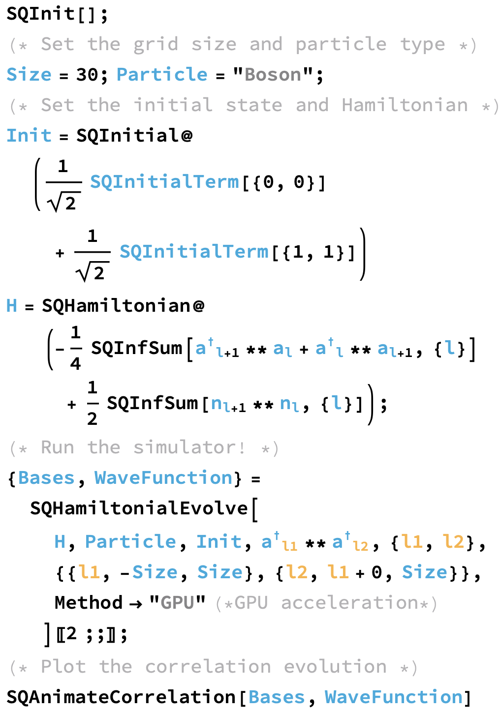
Example 2: 2D nearest-neighbor interaction walker

Here is a slightly more complicated example. The Hamiltonian with nearest-neighbor interaction is given by $$ \hat{H}=-J \sum_l\left( \ladup_{l+1}\laddown_l + \ladup_l\laddown_{l+1} \right) + U \sum_l n_{l+1} n_l $$ where $n_l$ is the particle number operator defined by $$ n_l = \ladup_l \laddown $$ and we have it defined in the package. The following code is all we need to simulate it.

Needs["CUDALink`"];
<< SQQW.wl
SQInit[];
(* Set the grid size and particle type *)
Size = 30; Particle = "Boson";
(* Set the initial state and Hamiltonian *)
Init = SQInitial @ (
  1/Sqrt[2] SQInitialTerm[{0, 0}]
 +1/Sqrt[2] SQInitialTerm[{1, 1}]
)
H = SQHamiltonian @ (
    -(1/4) SQInfSum[
      Subscript[SuperDagger[a], l + 1] ** Subscript[a, l] + 
      Subscript[SuperDagger[a], l] ** Subscript[a, l + 1], {l}]
    +1/2 SQInfSum[
      Subscript[n, l + 1] ** Subscript[n, l], {l}]
    );
(* Run the simulator! *)
{Bases, WaveFunction} =
  SQHamiltonialEvolve[
    H, Particle, Init, 
    Subscript[SuperDagger[a], l1] ** Subscript[SuperDagger[a], l2],
    {l1, l2}, {{l1, -Size, Size}, {l2, l1 + 0, Size}},
    Method -> "GPU"
   ][[2 ;;]];

It is hard to visualize the probability in this case, but we can plot the correlations:

References